A Data management platform (DMP) is a complex piece of software used to collect, store, classify, analyze, and distribute large quantities of data. It is a cornerstone technology for larger organizations when it comes to advertising data management, with rapidly increasing adoption. Data collection is a core capability of every data management platform. Being able to pull data from various disparate sources into one place may unlock enormous value. Typically, DMPs can ingest first-party data, second-party data from contracted partners, as well as third-party data from external providers.What differentiates various DMPs is the range of available data sources and integrations out of the box, data collection implementation, and speed of data transfer. The best DMPs have a large number of reliable (ideally lossless) and fast data integrations with other technology and data vendors. In addition, they offer an easy implementation with customization options.
Data Science and Governance
Introduction
In my role as a senior manager at the United Nations, I had the unique opportunity to lead a team of data scientists and architects on a groundbreaking climate change project.
The project aimed to provide actionable insights on the impact of climate change on agrobiodiversity and plant genetics. Utilizing a range of advanced sensors, we were able to capture a wealth of data, enabling us to make accurate models and analyses. This article delves into the specifics of the sensor technology used and the invaluable data collected for climate change assessment.
The Sensor Arsenal
Soil Moisture Sensors
These sensors were crucial in understanding how changing climate conditions affect soil water content, a key factor in plant health.
Temperature Sensors
We deployed these sensors to monitor both air and soil temperature, providing us with data to understand how temperature variations impact agrobiodiversity.
Humidity Sensors
These sensors helped us measure air humidity levels, which are critical for plant transpiration and overall health.
Light Sensors
Light sensors were used to monitor light intensity and duration, factors that directly influence plant growth and photosynthesis.
pH Sensors
Soil pH levels were continuously monitored to understand how soil acidity or alkalinity changes under different climate conditions.
Electrical Conductivity Sensors
These sensors assessed soil salinity, providing insights into how climate change could lead to soil degradation.
CO2 Sensors
Monitoring carbon dioxide levels helped us understand its impact on photosynthesis and plant growth.
Nutrient Sensors
These sensors measured essential soil nutrients like nitrogen, phosphorus, and potassium, offering insights into soil fertility.
Leaf Wetness Sensors
These sensors detected moisture levels on plant leaves, a critical factor in the spread of plant diseases.
Wind Speed Sensors
Wind conditions were monitored to understand how they affect plant transpiration and soil erosion.
Infrared Sensors
We used thermal imaging to assess plant health, providing a new layer of data for our analyses.
Spectral Sensors
These sensors captured specific wavelengths of light, providing detailed data on plant health and stress levels.
Data-Driven Insights
Utilizing these sensors, we collected a plethora of data types, including soil moisture levels, temperature variations, humidity levels, and more. This data was then processed and analyzed to create predictive models on the impact of climate change on agrobiodiversity.
The project led to significant improvements in our understanding of climate change impacts on agrobiodiversity. It also enabled interoperability with other public datasets, thanks to strong data quality policies that made the data fully FAIR (Findable, Accessible, Interoperable, and Reusable). The project required appropriate data modeling, definition of metadata schema, and data mining from 1.2 billion of GBIF records, creating a detailed data catalog to enable easy discovery and searchability of the insights.
AI Modeling for Climate Change Prediction
Below is a Python excerpt that demonstrates how to use a machine learning algorithm to predict climate change based on data coming from plant sensors.
The example uses a simple linear regression model for demonstration purposes.
The sensor data is assumed to be accessed using a JSON RESTful API.
pip install requests
pip install pandas
pip install tensorflow
import requests
import pandas as pd
import tensorflow as tf
from sklearn.model_selection import train_test_split
from sklearn.preprocessing import StandardScaler
from sklearn.metrics import mean_squared_error
# Function to fetch sensor data from RESTful API
def fetch_sensor_data(api_url):
response = requests.get(api_url)
if response.status_code == 200:
return response.json()
else:
return None
# Fetching sensor data
api_url = "http://XXX/api/sensor_data" # Replace with functioning API URL
sensor_data_json = fetch_sensor_data(api_url)
if sensor_data_json:
# Convert JSON to DataFrame
df = pd.DataFrame(sensor_data_json)
# Features and target variable
features = ['soil_moisture', 'temperature', 'humidity', 'CO2_levels']
target = 'climate_change_impact' # This is a hypothetical target variable
# Splitting the data into training and testing sets
X_train, X_test, y_train, y_test = train_test_split(df[features], df[target], test_size=0.2, random_state=42)
# Standardize the features
scaler = StandardScaler()
X_train_scaled = scaler.fit_transform(X_train)
X_test_scaled = scaler.transform(X_test)
# Initialize and train the model
model = tf.keras.Sequential([
tf.keras.layers.Dense(128, activation='relu', input_shape=(X_train_scaled.shape[1],)),
tf.keras.layers.Dense(64, activation='relu'),
tf.keras.layers.Dense(1)
])
model.compile(optimizer='adam', loss='mean_squared_error')
model.fit(X_train_scaled, y_train, epochs=50, batch_size=32)
y_pred = model.predict(X_test_scaled)
# Evaluate the model
mse = mean_squared_error(y_test, y_pred)
print(f"Mean Squared Error: {mse}")
else:
print("Failed to fetch sensor data.")
Predicting climate change effects
In the past I supported agrobiodiversity scientists demonstrating the causal effects of climate change on the living of the plants.
Scientists monitor and track more than 15.000 different plant species worldwide.
More than 1.300 Institutes worldwide collect “observations” of plants in a huge portal, the Global Biodiversity Information Facility GBIF https://www.gbif.org/
Today GBIF stores more than 1,3 billion of records catalogued using the data-standard Darwin Core, including observational data (GPS coordinates, altitude, etc.).
Challenges in statistics
How can you find evidence that climate changes is moving plants and/or change their dispersion on the territory. For example, some plants disappeared from where they were observed during ‘60s or appeared in new zones or at higher altitudes. Some other plants spread over mountains because the climate was more favorable due to the increase of temperature. Example: the plant Melampyrum nemorosum which lives in temperate climates has been observed now in Croatia mountains, which has very cold winters.
I collected the observation data needed, described data with descriptive statistics and performed regression analysis to find correlation among plants behavior and changes of the climate.
The Dataset
Datasets I worked on:
– Plants: GBIF portal, 250 million of observations made from 1920 to today
– Climate data from World Meteorological Organization GCOS: I used about 200k records of historical climate data observations
Variables considered:
– 152 variables from plants’ observations (Darwin Core data standard + Observational data)
– 13 variables from climate observations: precipitation, climate air temperature, humidity, wind speed, pressure, lightning, upper-air temperature, carbon dioxide (CO2), ozone, date, location (GPS coordinates)
Features
Data challenges
- Direct plants’ observations made in 60 years were affected by many quality issues:
- Human errors: name of the plants wrong, recorded date invalid, date invalid, geodetic datum invalid, elevation non-numeric or swapped, etc.
- Technology for observation changed, like the GPS tools (just few units in the 60s, today quite common with smartphones)
- Process to create observations changed: Initially scientists catalogued plants in printed forms; then scientists used Word documents, and, only in the last 30/40 years, relational databases have been adopted – I led a project to convert data from thousands printed forms to database of observations with metadata (presentation at TDWG 2010 conference)
- Undercoverage bias:
- Number of observations of plants in a specific area depends on the funds allocated to the Institutes in doing this process. Therefore, the presence of plants in a location depended on the number of observations made in that area. It means only some Institutes had good historical data.
- Scientists observed species only in some areas, probably close to their institutes, and at different times. This means I had to group by time the observations of plants in a map in order to consider which plants live in that area.
- Information bias:
- Each Institute uses its own set of tools and procedures to observe data. This means descriptive statistics are difficult to compare each other
- Observations happened at different seasons worldwide; in extreme climates (like cold winters or hot months) many plants naturally die so frequency of observations of course change.
- Climate data refers to the place where is located the meteorological station
- Time varying confounders: external factors to the climate change can modify the presence of plants in a zone, like pollution and human activities
Methodology for the problem
For some operations, like interpolation of climate data or calculation of the centroids of plants in a geographical map, I used the methodologies commonly used by agrobiodiversity scientists and climate specialists.
The methodology I followed was tailored for the data, and required in some transformations and assumptions:
- GROUPING OF OBSERVATIONS BY DATE: To calculate correctly descriptive measures, I grouped observations of plants by date of observation: all plants were considered “living organism” in the quarter of the year where observation was recorded. So, if a plant was observed in February 1998 then it became part of the group of plants living in the quarter January-March 1998 in that area.
- IDENTIFICATION OF CENTRES OF MASS OF SAMPLED PLANTS: I considered the geographical distribution of each sampled plant as concentrated in a single point, the centroid; for each plant sampled, I calculated also its mean and dispersion considering 10 hectares around its centroid. I considered the distance in meters centroids moved in a quarter. The hypothesis was that centroids moved because plants grow differently because of changes of climate factors.
- INTERPOLATION OF CLIMATE DATA: For the climate data, since the observations are done in meteorological stations, I performed interpolation of climate data to identify values in the exact location of the plants sampled. I used a deterministic interpolation algorithm called Inverse Distance Weighting (IDW), commonly used by climate scientists.
Unfortunately, I had to consider only those variables having good historical data, in the geographical areas identified after the sampling of the plants: humidity, temperature, pressure, precipitation.
Implementation
A standard process of statistic was followed, considering the quality issues and biases described above:
Multistage samplings of plants observations
Stage 1: Cluster sampling based on Institute names; only some Institutes collected good historical data
Stage 2: Stratified sampling based on qualitative variables of the plants (like kingdom, family name, genus name, taxonRank) – made by biologists
Stage 3: Systematic sampling – this avoided manipulation of the whole frame of Stage 2
The sample size resulted 1.2 million of samples of about 1250 plant species.
Definition of response variables
- Variation of GPS position of the centroids in meters (∆centroid) from quarter to quarter: the centroid is the centre of mass of the plants in a map, in a period of a quarter of year. I found the centroids using haversine formula with GPS coordinates
- Number of occurrences found in the area of 10 hectares around the centroid
- Variation of the Quartile Coefficient of Dispersion (∆QCD): the dispersion of plants in a region of 10 hectares around their centroids were measured by the Quartile Coefficient of Dispersion (QCD). Please note that the computation complexity for the QCD algorithm is excellent: O(n log n), n=number of units observed from a sampled plant
Inverse Distance Weighting (IDW) algorithm
- The dataframe was created locally considering the response variables above defined
- I accessed the historical observations of climate data from the GCOS institute and applied Inverse Distance Weighting (IDW) algorithm to interpolate the climate data in the exact location of the centroids of the sampled plants
- I determined the mean values of the climate data in that point in a quarter period (very time-consuming iterations; today accelerating adaptive inverse distance weighting algorithm could be used)
- I created then a dataframe joining data of sampled plants, climate data, observations data, date expressed in quarter/year
Data analysis
- Analysis of the dataframe and some findings:
- From time plots of samples, I found seasonality and some trends on number of plants in a region and their spread in that region
- With Polar seasonal plots and scatterplot matrices, I found good correlations of some groups of plants with the climate data: with the help of biologists, we identified group of plants which responded more to variations of climate data. Example: plants that live at high altitudes or plants with good autochthone resilience showed high correlation of dispersion with temperature and humidity
- Forecasts from regression model highlighted that at ground level plants should increase dispersion in their region (∆QCD) and their occurrences in their region should drastically drop
- Some plants found the habitat at different locations: this was evident mostly in dried areas where the ∆centroid values were higher
- Putting altitude of observations as a response variable, I found some plants changed their altitude because of the change of climate in their region. So even if their dispersion in the territory was low (∆QCD) they actually spread vertically over mountains and hills
Getting data
- Data accessed and manipulated via dedicated RESTFUL API of the data provider GBIF
- Data engineering of local datasets done in dedicated on-premises servers
- Development language: python and some R scripts, T-SQL for some data manipulation functions
- Languages for data engineering: SQL and stored procedures in Microsoft SQL Server
- Geographical tools: ArcGIS, google maps
- Development tools: Eclipse
1) Ridge Regression with Scikit-Learn using a closed-form solution:
from sklearn.linar_model import Ridge
ridge_reg = Ridge(alpha=1, solver=”cholesky”)
ridge_reg.fit(X, y)
ridge_reg.predict([[1.6]])
2) Ridge Regression with Scikit-Learn using Stochastic Gradient Descent:
sgd_reg = SGDRegressor (penalty=”08″)
sgd_reg.fit(X, y.ravel())
sgd_reg.predict([[1.6]])
Curvilinear Component Analysis (CCA) is a technique for reducing the dimensionality of a dataset while preserving its local structure. It is an extension of the well-known Principal Component Analysis (PCA) method but is designed to handle non-linear relationships between the features. CCA uses a more localized criterion than PCA, allowing it to better capture the local topology of the data. The goal of CCA is to find a lower-dimensional representation of the data that maintains the important structure of the original dataset. This makes it particularly useful for representing non-linear patterns in the data.
Some examples to help illustrate the concept:
- Image compression: CCA can be used to reduce the dimensionality of an image without losing important details. For example, in a picture of a face, CCA can identify and preserve the non-linear relationships between the features, such as the curve of the cheek or the slope of the nose, while reducing the number of pixels.
- Speech recognition: CCA can also be used in speech recognition systems to extract the most relevant features from audio signals. The technique can identify non-linear relationships between the different sound frequencies, allowing for a more accurate representation of the speech.
- Data visualization: CCA can be used to visualize high-dimensional data in two or three dimensions for easier interpretation. The technique can help to reveal patterns and relationships in the data that might not be immediately apparent in the raw data.
In all these examples, CCA is useful because it allows for a more effective representation of the data while preserving its underlying structure, making it easier to analyze and understand.
Some business cases where Curvilinear Component Analysis (CCA) can be applied:
- Customer segmentation: CCA can be used to segment customers based on their purchasing behavior. The technique can identify non-linear relationships between the different customer features, such as their demographics and purchasing history, allowing for a more accurate representation of the customer segments.
- Fraud detection: CCA can also be used in fraud detection systems to extract relevant features from transaction data. The technique can identify non-linear relationships between the different features, such as the time of day and the location of the transaction, allowing for more accurate detection of fraudulent activity.
- Marketing analytics: CCA can be used to analyze customer behavior and preferences to inform marketing strategies. The technique can help to identify non-linear relationships between customer demographics, purchasing history, and other relevant features, allowing for a more effective targeting of marketing campaigns.
Using CCA (or any other dimensionality reduction technique) can lead to cost savings by reducing the amount of data that needs to be processed and stored, reducing the computational resources required for analysis, and improving the accuracy of the results, which can lead to more efficient and effective decision-making.
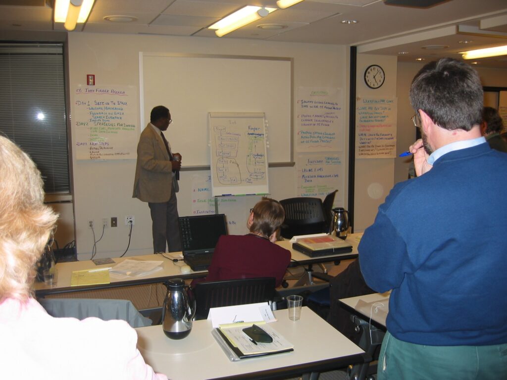
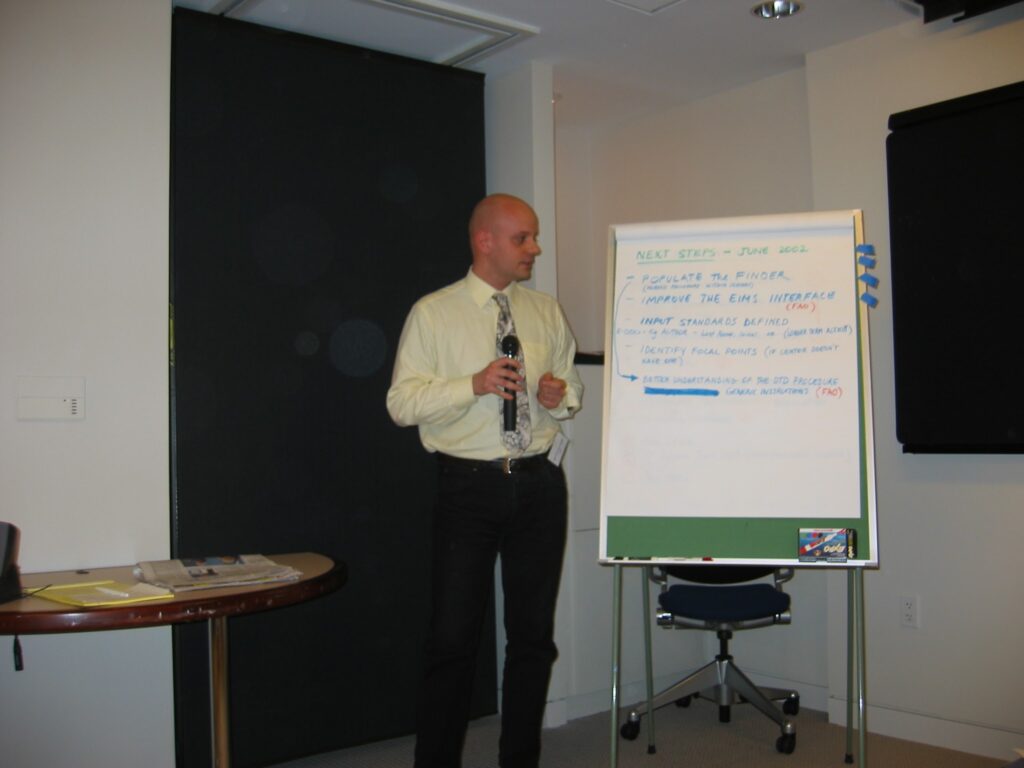
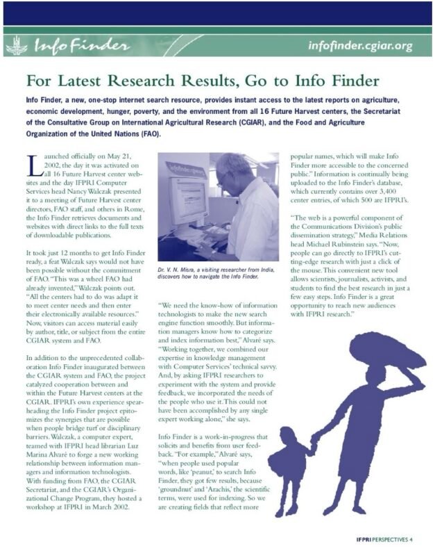
InfoFinder Launch at IFPRI, Washington DC (USA)
A new online search tool for agricultural and environmental information has been unveiled by a consortium of global food and environmental research organizations, marking a significant advancement in digital resource access. This innovative platform was introduced in anticipation of the forthcoming “World Food Summit: Five Years Later” in Rome, underscoring its pivotal role in transforming access to specialized agricultural and development data.
The tool, named Info Finder and accessible via http://infofinder.cgiar.org, represents a concerted effort among several key organizations. These include the World Agricultural Information Center, operated under the auspices of the Food and Agriculture Organization of the United Nations; Future Harvest Centers across the globe; and the Consultative Group on International Agricultural Research (CGIAR).
Francisco Reifschneider, the Director of CGIAR, emphasized the exponential growth of agricultural information available online and pointed out that Info Finder significantly facilitates swift access to an extensive repository of agricultural knowledge produced by the Future Harvest Centers. The system leverages FAO’s proprietary technologies, employing common standards such as keywords from the Agrovoc agricultural thesaurus to streamline the search process for online information.
In the context of this collaboration, Francisco Perez-Trejo, manager at the World Agricultural Information Center, highlighted the FAO’s commitment to enhancing the reach, impact, and sustainability of agricultural information management systems through strategic partnerships.
The CGIAR, established in 1971, stands at the forefront of this endeavor as a premier development partnership. It fosters a comprehensive knowledge network among 16 Future Harvest Centers, dedicated to addressing the pressing challenges of agriculture and development.
Massimo Buonaiuto’s participation in this initiative underscores the critical role of leading data science and digital transformation experts in advancing agricultural research and information dissemination. Through such collaborative efforts, the global community moves closer to achieving sustainable agricultural practices and food security.


Some documentation